AstroFV

As a user, you can use AstroFV to perform simulation of an astrophysical application. The following simulations are currently supported. Please click on the relevant one:

Relativistic Shock Tube Problem (RSTP) in 1-D

RSTP

Introduction

Astrophysical scenarios involving relativistic flows occur in several phenomenon, most notably in the jets in extragalactic radio sources associated with active galactic nuclei. Similar to shock wave phenomenon in classical Newtonian fluid mechanics, strong shocks are a common feature in such astrophysical scenarios. Numerical simulations are therefore needed to study the formation, evolution and interaction of shock waves in relativistic fluids.

Relativistic shock tube problem (RSTP) involves the decay of an initially discontinuous two fluids into three elementary wave structures: a shock, a contact, and a rarefaction wave.

Governing Equations

This application considers the hydrodynamics model of a perfect fluid. The model is thus given by the hyperbolic system of conservation laws of the relativistic hydrodynamics.

Following Hujeirat and Font, the 1-dimensional hydrodynamical system in Minkowski space can be reformulated in terms of dynamical variables $D, M_{\mu}, E_{d}$ as:

$\frac{\partial D}{\partial t} + \frac{\partial (DV^{x})}{\partial x} = 0$

$\frac{M_{x}}{\partial t} + \frac{\partial (M_{x}V^{x})}{\partial x} = -\frac{\partial P}{\partial x}$

$\frac{E^{d}}{\partial t} + \frac{\partial (E^{d}V^{x})}{\partial x} = -(\gamma - 1)\frac{E^d}{u^t} \lbrack \frac{\partial u^t}{t} + \frac{\partial V^x}{\partial x}\rbrack$

where we define

$D = \rho u^t$ = Relativistic Density

$M_{x} = \rho h u_{x}u^t$ = Momentum

$E^{d} = \rho \epsilon u^t$ = Total energy (assuming conservation of mechanical energy)

$V^x = \frac{u^x}{u^t}$ = Transport Velocity

$\sqrt{-g} = 1$ in Minkowski space

$u^{\mu}$ = four-velocity of the fluid

$\rho$ = rest mass density in locally intertial reference frame

$h = 1 + \epsilon + \frac{p}{\rho}$ = relativistic specific enthalpy

$\epsilon$ = specific internal energy

$p & = $(\gamma - 1)\rho \epsilon$ = pressure of ideal gas

The above equations are the desired equations which can be solved for the following cases:

Adiabatic conditions
- isothermal gas (specified with gamma = 0)
- non-isothermal gas with gamma = User defined (practically 4/3, 5/3, 2)
Initial conditions

$\rho_{init}$ = User input

$p_{init}$ = User input

$D_{init}$ = User input

$M^{x}_{init}$ = User input

$V^{x}_{init}$ = User input

$E^{d}_{init} = \frac{p_{init}}{\gamma - 1}$
Remarks
- The hydrodynamical system represents a coupled set of non-linear advection equations
- If fluid is considered isothermal, h~1 and the equation in E should be ignored (need not solved)
- For non-isothermal case, Dh = D + $\gamma E^d$
- Dh ~ D for isothermal case
- $M_{t}^2 = M_{x}^2 + (Dh)^2$
- $u^{t} = \frac{M_{t}}{Dh}$
- $u^{x} = \frac{M_{x}}{Dh}$
- $V^{x} = \frac{u^{x}}{u^{t}} = \frac{M_{x}}{M_{t}}$
- $\rho = \frac{D}{u^{t}}$
- $p = \frac{E^{d}(\gamma-1)}{u^{t}}$
- To get $E^{d}_{init}$
  
  we have used that
  
  $E^{d} = \frac{u^{t}p}{(\gamma - 1)}$ and $u^{t} = \frac{M^{t}}{Dh} = \frac{\sqrt{M_{x}^2+(Dh)^2}}{Dh}$

Numerical techniques

Spatial discretization

Using first order upwinding with constant grid size

Temporal discretization

Constant grid size is used

We use cell centered FV discretization for Density and Momentum conservation and vertex centered FV discretization for Total energy. This is shown below FV Cells for RSTP

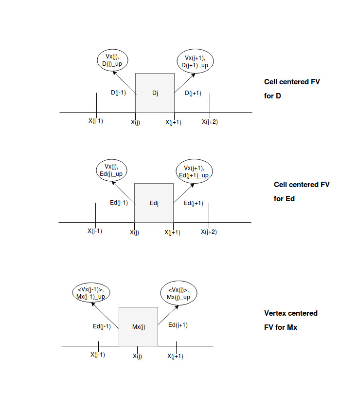
For vertex centered approach, the transport velocity at FV cell surface is taken as the mean value across the boundary. i.e

$\qquad \langle V_{j-1}^x \rangle = \frac{V_{j-1}^x + V_{j}^x}{2} \qquad \langle V_{j}^x \rangle = \frac{V_{j}^x + V_{j+1}^x}{2}$

The upwind flux across the FV cell surfaces is defined as:

$D_{j}^{up} = \begin{cases} D_{j} \quad \text{ if } V_{j}^x \leq 0 \\ D_{j-1} \quad \text{ if } V_{j}^x > 0 \end{cases}$

$Ed_{j}^{up} = \begin{cases} Ed_{j} \quad \text{ if } V_{j}^x \leq 0 \\ Ed_{j-1} \quad \text{ if } V_{j}^x > 0 \end{cases}$

$\begin{cases} Mx_{j} \quad \text{ if } \langle V_{j}^x \rangle \leq 0 \\ Mx_{j-1} \quad \text{ if } \langle V_{j}^x \rangle > 0 \end{cases}$

Discretized equations using Explicit Euler

$D_{j}^{n+1} = D_{j}^{n} - \Delta t \left( \frac{D_{j}^{up}V_{j+1}^x - D_{j}^{up}V_{j}^x}{\Delta x} \right)^{n}$

$Mx_{j}^{n+1} = Mx_{j}^{n} - \Delta t \left( \frac{Mx_{j}^{up}\langle V^{x} \rangle_{j} - Mx_{j-1}^{up} \langle V^{x} \rangle_{j-1}}{\Delta x} \right)^{n} - \Delta t \left( \frac{p_{j}-p_{j-1}}{\Delta x} \right)$

$Ed_{j}^{n+1} = Ed_{j}^{n} - \Delta t \left( \frac{Ed_{j}^{up}V_{j+1}^x - Ed_{j}^{up}V_{j}^x}{\Delta x}\right)^{n} - \Delta t \left( (\gamma - 1) \left( \frac{Ed}{u^t}\right)^n \left( \frac{(u^t)^{n+1}-(u^t)^n}{\Delta t} + \frac{V_{j+1}^x - V_{j}^x}{\Delta x }\right) \right)$

Discretized equations using Implicit Euler

The paramater $\alpha$ controls the implicit scheme. Value 1.0 implies Implicit Euler. Other useful values like 0.5 which imply Crank-Nicholson are for future use.

The 3 set of equations can be written as:

$\frac{D_{j}^{n+1} - D_{j}^{n}}{\Delta t} + \alpha \left( \frac{D_{j+1}^{up,n+1}V_{j+1}^{x,n+1} - D_{j}^{up,n+1}V_{j}^{x,n+1}}{\Delta x} \right) + (1-\alpha) \left( \frac{D_{j+1}^{up,n}V_{j+1}^{x,n} - D_{j}^{up,n}V_{j}^{x,n}}{\Delta x} \right) = 0$

$\frac{M_{j}^{n+1} - M_{j}^{n}}{\Delta t} + \alpha \left( \frac{M_{j}^{up,n+1}\langle V_{j}^{x,n+1} \rangle - M_{j-1}^{up,n+1} \langle V_{j-1}^{x,n+1} \rangle}{\Delta x} \right) + (1-\alpha) \left( \frac{M_{j}^{up,n}\langle V_{j}^{x,n} \rangle - M_{j-1}^{up,n} \langle V_{j-1}^{x,n} \rangle}{\Delta x} \right) = -\alpha \left( \frac{p_{j}^{n+1}-p_{j-1}^{n+1}}{\Delta x} \right) -(1-\alpha) \left( \frac{p_{j}^{n+1}-p_{j-1}^{n+1}}{\Delta x} \right)$

$\frac{E_{j}^{n+1} - E_{j}^{n}}{\Delta t} + \alpha \left( \frac{E_{j+1}^{up,n+1}V_{j+1}^{x,n+1} - E_{j}^{up,n+1}V_{j}^{x,n+1}}{\Delta x} \right) + (1-\alpha) \left( \frac{E_{j+1}^{up,n}V_{j+1}^{x,n} - E_{j}^{up,n}V_{j}^{x,n}}{\Delta x} \right) = (\gamma - 1) \frac{E_{j}^{n+1}}{u^{n+1}} \left( \frac{u^{n+1} - u^{n}}{\Delta t} + \frac{V_{j+1}^{n+1}-V_{j}^{n+1}}{\Delta x} \right )$

which when re-arranged gives a tridiagonal system of equations as follows:

$\text{ if } V_{j}^x > 0$ , then

$D_{j-1}^{n+1} \left( \frac{-\alpha V_{j}^{x,n+1}}{\Delta x} \right) + D_{j}^{n+1} \left( \frac{1}{\Delta t} + \frac{\alpha V_{j+1}^{x,n+1}}{\Delta x} \right) + D_{j+1}^{n+1} (0) = \frac{D_{j}^{n}}{\Delta t} - (1-\alpha) \left(\frac{D_{j}^{n}V_{j+1}^{x,n} - D_{j-1}^{n}V_{j}^{x,n}}{\Delta x} \right)$

$M_{j-1}^{n+1} \left( \frac{-\alpha \langle V_{j-1} \rangle ^{x,n+1}}{\Delta x} \right) + M_{j}^{n+1} \left( \frac{1}{\Delta t} + \frac{\alpha \langle V_{j} \rangle ^{x,n+1}}{\Delta x} \right) + M_{j+1}^{n+1} (0) = \frac{M_{j}^{n}}{\Delta t} - (1-\alpha) \left(\frac{M_{j}^{n}\langle V_{j} \rangle ^{x,n} - M_{j-1}^{n}\langle V_{j-1} \rangle ^{x,n}}{\Delta x} \right) - \alpha \left( \frac{p_{j}^{n+1}-p_{j-1}^{n+1}}{\Delta x} \right) - (1-\alpha) \left( \frac{p_{j}^{n}-p_{j-1}^{n}}{\Delta x} \right)$

$E_{j-1}^{n+1} \left( \frac{-\alpha V_{j}^{x,n+1}}{\Delta x} \right) + E_{j}^{n+1} \left( \frac{1}{\Delta t} + \frac{\alpha V_{j+1}^{x,n+1}}{\Delta x} - \frac{\gamma - 1}{u^{n+1}} \left( \frac{\partial u}{\partial t} + \frac{V_{j+1}^{x,n+1}-V_{j}^{x,n+1}}{\Delta x} \right) \right) + E_{j+1}^{n+1} (0) = \frac{E_{j}^{n}}{\Delta t} - (1-\alpha) \left(\frac{E_{j}^{n}V_{j+1}^{x,n} - E_{j-1}^{n}V_{j}^{x,n}}{\Delta x} \right)$

and $\text{ if } V_{j}^x \leq 0$ , then

$D_{j-1}^{n+1}(0) + D_{j}^{n+1} \left( \frac{1}{\Delta t} - \frac{\alpha V_{j}^{x,n+1}}{\Delta x} \right) + D_{j+1}^{n+1} \left( \frac{\alpha V_{j+1}^{x,n+1}}{\Delta x} \right) = \frac{D_{j}^{n}}{\Delta t} - (1-\alpha) \left(\frac{D_{j+1}^{n}V_{j+1}^{x,n} - D_{j}^{n}V_{j}^{x,n}}{\Delta x} \right)$

$M_{j-1}^{n+1} (0) + M_{j}^{n+1} \left( \frac{1}{\Delta t} - \frac{\alpha \langle V_{j-1} \rangle ^{x,n+1}}{\Delta x} \right) + M_{j+1}^{n+1} \left( \frac{\alpha \langle V_{j} \rangle ^{x,n+1}}{\Delta x} \right) = \frac{M_{j}^{n}}{\Delta t} - (1-\alpha) \left(\frac{M_{j+1}^{n}\langle V_{j} \rangle ^{x,n} - M_{j}^{n}\langle V_{j-1} \rangle ^{x,n}}{\Delta x} \right) - \alpha \left( \frac{p_{j}^{n+1}-p_{j-1}^{n+1}}{\Delta x} \right) - (1-\alpha) \left( \frac{p_{j}^{n}-p_{j-1}^{n}}{\Delta x} \right)$

$E_{j-1}^{n+1} (0) + E_{j}^{n+1} \left( \frac{1}{\Delta t} - \frac{\alpha V_{j}^{x,n+1}}{\Delta x} - \frac{\gamma - 1}{u^{n+1}} \left( \frac{\partial u}{\partial t} + \frac{V_{j+1}^{x,n+1}-V_{j}^{x,n+1}}{\Delta x} \right) \right) + E_{j+1}^{n+1} \left( \frac{\alpha V_{j+1}^{x,n+1}}{\Delta x} \right) = \frac{E_{j}^{n}}{\Delta t} - (1-\alpha) \left(\frac{E_{j+1}^{n}V_{j+1}^{x,n} - E_{j}^{n}V_{j}^{x,n}}{\Delta x} \right)$

Remarks

The dependence on values from (n+1)th iteration for Vx and P are handled by using an iterative procedure. This is explained in pseudo code below:

  Expectation: We are in iteration n, given values of step n we want to calculate values for n+1
  Input: Dn, Vn, Mn, Edn, Pn as the values from step n, iter_count as number of sub-iterations
  Procedure:
  	Set:
     V* = Vn
     P* = Pn
 Loop: Execute the below sub-iteration for iter_count:
     #Solve the 3 equations
     D' = f1(Dn,Vn,V*)
     M' = f2(Mn,Vn,V*,P*)
     E' = f3(En,Vn,V*)
   		
     #Update phase
     V* = update_Vx(D',M')
     P* = update_pressure(D',E')
   		
     Repeat loop
   		
 Finally:
     Vn+1 = V*
     Pn+1 = P*
     Dn+1 = D'
     Mn+1 = M'
     En+1 = E'

Key Data structures

Parameters

  class RSTPExplicitParams(Params):
     def __init__(self,ncells,gamma=0,cfl=1.0):
         Params.__init__(self,"explicit") 
         self.gamma = gamma
         self.cfl = cfl
         self.ncells = ncells
         self.fv_boundary_strategy = None
   
  class RSTPImplicitParams(Params):
     def __init__(self,ncells,alpha,gamma=0,iter_count=1,cfl=0.50):
         Params.__init__(self,"implicit") 
         self.gamma = gamma
         self.ncells = ncells
         self.alpha = alpha
         self.fv_boundary_strategy = None        
         self.cfl = cfl #This is used to define time step size
         self.iter_count = iter_count

These are used to define parameters for Explicit Euler time integration and Implicit time integration.

gamma = 0 defines isothermal gas

Time limits are default [0,1] and spatial limits are default [0,1].

Spatial grid size is automatically chosen by dividing spatial limit by ncells.

Temporal grid size is automatically derived from spatial grid size by using CFL parameter. delta_t = self.params.cfl*delta_x

Example:

   eparams = RSTPExplicitParams(1000,0,0.25) #isothermal gas, CFL=0.25
   iparams = RSTPImplicitParams(1000,1.0,0.0,2,0.7) #isothermal gas, Implicit Euler solver, iter_count=2, cfl=0.7

Initial Values

class RSTPIV(InitialValues):
 def __init__(self,Vx,Mx,D,Rho):
     self.Vx = Vx
     self.Mx = Mx
     self.D = D
     self.Rho = Rho

Used to provide initial values. The initial values are provided as a list for the two discontinuous fluids.

Example:

   iv = RSTPIV(Vx=[0,0],Mx=[0,0],D=[1,10**-2],Rho=[1,10**-2])

Usage examples

###### Solve RSTP using Explicit Euler Number of FV cells = 1000, gamma = 4/3, CFL = 0.25

     eparams = RSTPExplicitParams(1000,4/3,0.25) 
     eparams.set_fig_path('./figs/')
     eparams.fv_boundary_strategy = FVTransverse #Default 
     eiv = RSTPIV(Vx=[0,0],Mx=[0,0],D=[1,10**-2],Rho=[1,10**-2])
     ebv = RSTPBV()
     test_explicit = RSTPTest(1,eparams,eiv,ebv,ode_strategy=ODEExplicit)
     test_explicit.solve()

###### Solve RSTP using Implicit Euler Number of FV cells = 1000, gamma = 4/3, CFL = 0.7, no of subiterations = 2

     iparams = RSTPImplicitParams(1000,1.0,4/3,2,0.7)
     iparams.set_fig_path('./figs/')
     iparams.fv_boundary_strategy = FVTransverse #Default 
     iiv = RSTPIV(Vx=[0,0],Mx=[0,0],D=[1,10**-2],Rho=[1,10**-2])
     ibv = RSTPBV()
     test_implicit = RSTPTest(2,iparams,iiv,ibv,ode_strategy=ODEImplicit)
     test_implicit.solve()

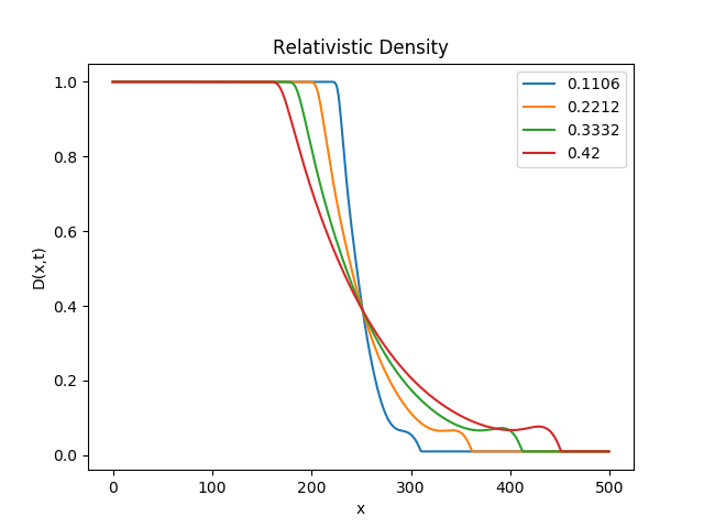
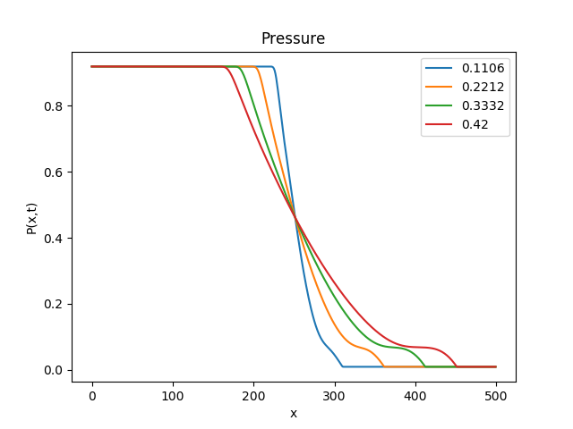
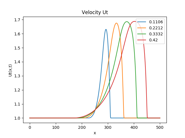
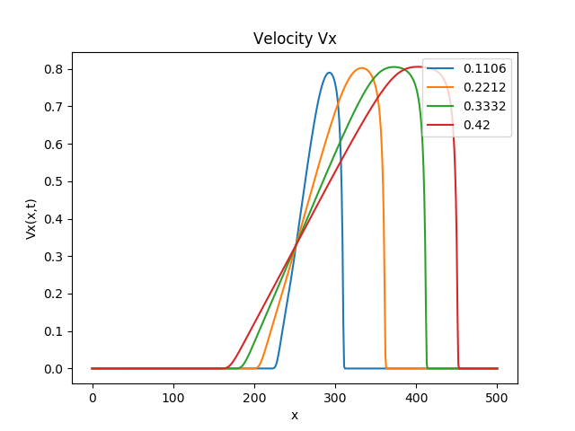
#### Output The output is generated as a set of 4 image files in the same directory as provided in set_fig_path() API.

The 4 image files correspond to plot of spatial variable x against Relativistic Density (D), Pressure(P), Lorentz factor ( $u^{t}$ ) and Transport Velocity ( $V^x$ ) respectively

An example is shown below: RSTP Relativistic Density RSTP Pressure RSTP Lorentz factor RSTP Transport Velocity